程序返回一个 5x5 的单位矩阵
    A = [[1, 0, 0, 0, 0],
         [0, 1, 0, 0, 0],
         [0, 0, 1, 0, 0],
         [0, 0, 0, 1, 0],
         [0, 0, 0, 0, 1]]
    A = np.eye(5)
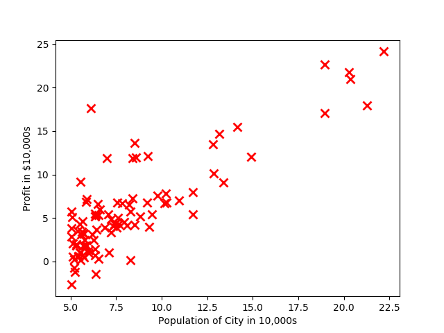
然后绘制给定数据x与y的图像
计算线性回归的代价
前面有系数2的原因是下面求梯度是对每个变量求偏导,2可以消去
注意这里的X是真实数据前加了一列1,因为有theta(0)
梯度下降算法学习参数theta
代价函数对 $\theta_{j}$ 求偏导:
theta更新为:
$\alpha$ 为学习速率,控制梯度下降的速度,一般取0.01,0.03,0.1,0.3…..
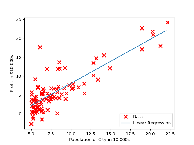
打印theta[0], theta[1]:-3.630291,1.166362
在绘制数据点的基础上绘制回归得到直线
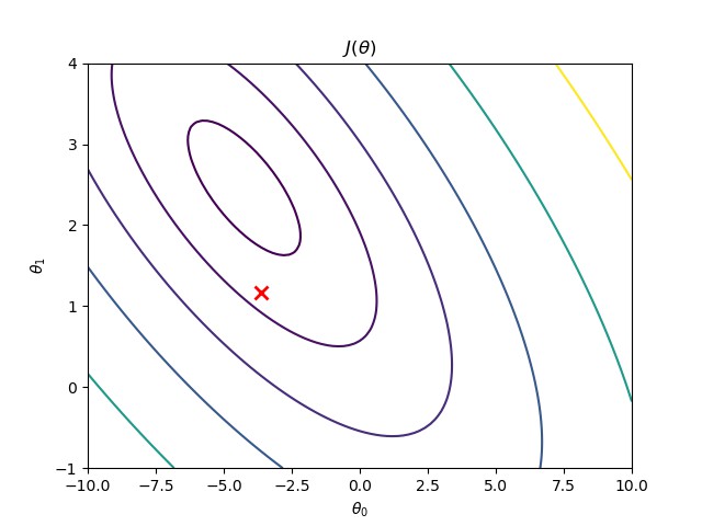
可视化代价函数
本文涉及到的数据集:PRML_LR_data.txt
程序代码
# coding: utf-8

# If you use python 2, uncomment the following line.
# from __future__ import print_function

import numpy as np
import matplotlib.pyplot as plt


def warm_up_exercise():
    """热身练习"""
    A = None
    # ====================== 你的代码 ==========================
    # 在下面加入你的代码,使程序返回一个 5x5 的单位矩阵
    A = [[1, 0, 0, 0, 0],
    	 [0, 1, 0, 0, 0],
    	 [0, 0, 1, 0, 0],
    	 [0, 0, 0, 1, 0],
    	 [0, 0, 0, 0, 1]]

    # =========================================================
    return A


def plot_data(x, y):
    """绘制给定数据x与y的图像"""
    plt.figure()
    # ====================== 你的代码 ==========================
    # 绘制x与y的图像
    # 使用 matplotlib.pyplt 的命令 plot, xlabel, ylabel 等。
    # 提示:可以使用 'rx' 选项使数据点显示为红色的 "x",
    #       使用 "markersize=8, markeredgewidth=2" 使标记更大

    # 给制数据
    plt.plot(x, y, 'rx', markersize=8, markeredgewidth=2)#or圆点
    # 设置y轴标题为 'Profit in $10,000s'
    plt.ylabel('Profit in $10,000s')
    # 设置x轴标题为 'Population of City in 10,000s'
    plt.xlabel('Population of City in 10,000s')
    # =========================================================
    plt.show()


def compute_cost(X, y, theta):
    """计算线性回归的代价"""
    m = len(y)
    J = 0.0
    # ====================== 你的代码 ==========================
    # 计算给定 theta 参数下线性回归的代价
    # 请将正确的代价赋值给 J

    # 注意:在主函数中将行向量变列向量
    J = (1.0/(2*m))*np.sum(np.square(X.dot(theta)-y))
    # J = (np.transpose(X*theta-y))*(X*theta-y)/(2*m) #计算代价J
    # =========================================================
    return J


def gradient_descent(X, y, theta, alpha, num_iters):
    """执行梯度下降算法来学习参数 theta"""
    m = len(y)
    J_history = np.zeros((num_iters,))

    for iter in range(num_iters):
        # ====================== 你的代码 ==========================
        # 计算给定 theta 参数下线性回归的梯度,实现梯度下降算法
        deltaTheta = (1.0/m)*(X.T.dot(X.dot(theta)-y))
        # =========================================================
        # 将各次迭代后的代价进行记录
        J_history[iter] = compute_cost(X, y, theta)
        theta = theta-alpha*deltaTheta
        # ==========================================================
    return theta, J_history


def plot_linear_fit(X, theta):
    """在绘制数据点的基础上绘制回归得到直线"""
    # ====================== 你的代码 ==========================
    # 绘制x与y的图像
    # 使用 matplotlib.pyplt 的命令 plot, xlabel, ylabel 等。
    # 提示:可以使用 'rx' 选项使数据点显示为红色的 "x",
    #      使用 "markersize=8, markeredgewidth=2" 使标记更大
    #      使用"label=<your label>"设置数据标识,
    #      如 "label='Data'" 表示原始数据点
    #      "label='Linear Regression'" 表示线性回归的结果

    # 绘制数据
    xx = np.arange(5,23)
    yy = theta[0]+xx*theta[1]
    plt.plot(X[:,1], y, 'rx', label='Data', markersize=8, markeredgewidth=2)
    plt.plot(xx,yy,label='Linear Regression')
    # 使用 legned 命令显示图例,图例显示位置为 "loc='lower right'"
    plt.legend(loc='lower right')
    # 设置y轴标题为 'Profit in $10,000s'
    plt.ylabel('Profit in $10,000s')
    # 设置x轴标题为 'Population of City in 10,000s'
    plt.xlabel('Population of City in 10,000s')
    # =========================================================
    plt.show()


def plot_visualize_cost(X, y, theta_best):
    """可视化代价函数"""

    # 生成参数网格
    theta0_vals = np.linspace(-10, 10, 101)
    theta1_vals = np.linspace(-1, 4, 101)
    t = np.zeros((2, 1))
    J_vals = np.zeros((101, 101))
    for i in range(101):
        for j in range(101):
            # =============== 你的代码 ===================
            # 加入代码,计算 J_vals 的值
            J_vals[i,j] =  (1.0/(2*len(y)))*np.sum(np.square(theta0_vals[i]+X.dot(theta1_vals[j])-y))
            # pass                # 完成你的代码后请删除此行
            # ===========================================
    '''
    # 二维曲线
    X=X[:,1]
    #theta2=np.arange(-10,11,0.01)
    theta2=np.linspace(-10,11,101)
    n=y.size
    J=np.zeros(theta2.size)
    for i in np.arange(theta2.size):
        J[i]=(1.0/(2*n))*np.sum(np.square(X.dot(theta2[i])-y))
    plt.plot(theta2, J)
    '''

    # 绘制等高线
    plt.figure()
    plt.contour(theta0_vals, theta1_vals, J_vals,
                levels=np.logspace(-2, 3, 21))
    plt.plot(theta_best[0], theta_best[1], 'rx',
            markersize=8, markeredgewidth=2)
    plt.xlabel(r'$\theta_0$')
    plt.ylabel(r'$\theta_1$')
    plt.title(r'$J(\theta)$')
    plt.show()


if __name__ == '__main__':
    print('Running warm-up exercise ... \n')
    print('5x5 Identity Matrix: \n')
    A = warm_up_exercise()
    print(A)

    print('Plotting Data ...\n')
    data = np.loadtxt('PRML_LR_data.txt', delimiter=',')
    x, y = data[:, 0], data[:, 1]
    m = len(y)
    plot_data(x, y)
    plt.show()

    print('Running Gradient Descent ...\n')

    # Add a column of ones to x

    X = np.ones((m, 2))
    X[:, 1] = data[:, 0]
    # 将行向量转换为列向量
    # X = np.c_[np.ones(data.shape[0]), data[:,0]]
    # y = np.c_[data[:, 1]]
    X = np.c_[X]
    y = np.c_[y]

    # initialize fitting parameters
    theta = np.zeros((2, 1))

    # Some gradient descent settings
    iterations = 1500
    alpha = 0.01

    # compute and display initial cost
    # Expected value 32.07
    J0 = compute_cost(X, y, theta)
    print(J0)

    # run gradient descent
    # Expected value: theta = [-3.630291, 1.166362]
    theta, J_history = gradient_descent(X, y,theta, alpha,iterations)
    print('Theta found by gradient descent:')
    print('%f %f' % (theta[0], theta[1]))
    #print('theta:', theta.ravel())

    plot_linear_fit(X, theta)
    plt.show()

    plot_visualize_cost(X, y, theta)
    plt.show()