逻辑回归
优点:计算代价不高,易于理解实现
缺点:容易欠拟合,分类精度可能不高
适用数据类型:数值型和标称型数据
为了实现逻辑回归,我们在每个特征上乘以一个回归系数,然后把所有的结果值相加,将这个总和代入Sigmoid函数中,进而得到一个0-1范围之间的数值。任何大于0.5的分为1类,小于0.5归为0类。最佳回归系数多少?
这里将实现逻辑回归算法,并将之应用于两个数据集:Logistic_data1.txt和Logistic_data2.txt
需要实现的函数:
- plot_data: 绘制二维的分类数据
- sigmoid: sigmoid函数
- cost_function: 逻辑回归的代价函数
- predict: 逻辑回归的预测函数
- cost_function_reg: 逻辑回归带正则化项的代价函数
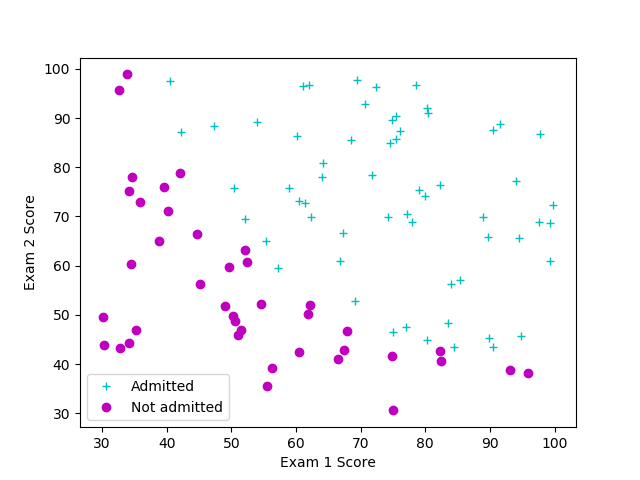
数据可视化
    pos = y == 1
    neg = y == 0
    plt.plot(X[pos, 0], X[pos, 1], 'c+', label="Admitted")
    plt.plot(X[neg, 0], X[neg, 1], 'mo', label="Not admitted")
sigmoid函数
逻辑回归的假设模型:
其中函数$g(·)$是sigmoid函数,定义为:
代价函数与梯度
现在需要实现逻辑函数回归的代价函数及其梯度。逻辑回归的代价函数为:
对应的梯度向量各分量为:
传入初始参数,cost_function的代价约为0.693。
使用fmin_cg学习模型参数
使用scipy.optimize.fmin_cg函数实现代价函数$J(\theta)$的优化,得到最佳参数$\theta^{*}$。
调用该函数的方法如下:
    ret = op.fmin_cg(cost_function,
        theta_initial,
        fprime = cost_gradient,
        args = (X,y),
        maxiter = 200,
        full_output = True)
其中cost_function为代价函数,theta_initial为需要优化的参数的初始值,fprime=cost_gradient给出了代价函数的梯度,args=(X,y)给出了需要优化的函数与对应的梯度计算所需要的其他参数,maxiter=400给出了最大迭代次数,full_output=True则指明该函数除了输出优化得到的参数theta_opt外,还会返回最小的代价函数值cost_min等内容。对一组参数得到的代价约为0.203(cost_min)。
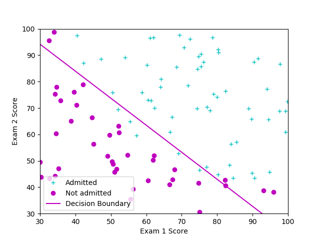
评估逻辑回归模型
在获得模型参数后,可以使用模型预测一个学生能够被大学录取的几率。如果某学生考试一的成绩为45,考试二的成绩为85,能够得到录取几率约为0.776。
predict函数输出”1”或”0”,通过计算分类正确的样本百分数,可以得正确率。
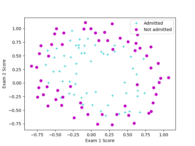
正则化的逻辑回归
调用函数plot_data可视化第二组数据。
特征变换:
创建更多的特征是充分挖掘数据中的信息的一种有效手段。该函数map_feature中,将数据映射为6阶多项式的所有项。
逻辑回归的代价函数为:
对应的梯度向量各分量为:
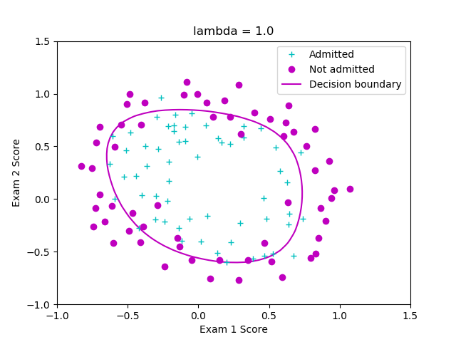
如果将参数 初始化为全零值,相应的代价函数约为0.693,。可以使用与前述无正则化项类似的方法实现梯度下降,获得优化后的参数$\theta^{*}$。
可以调用plot_decision_boundary函数来查看最终得到的分类面。建议你调整正则化项的系数,分析正则化对分类面的影响。
程序代码
# -*- encoding: utf-8 -*-

from __future__ import print_function

import numpy as np
import scipy.optimize as op
import matplotlib.pyplot as plt


def plot_data(X, y):
    """This function plots the data points X and y into a new figure.
    It plots the data points with red + for the positive examples,
    and blue o the negative examples. X is assumed to be a Mx2 matrix.
    """
    plt.figure()
    # ====================== YOUR CODE HERE ======================
    pos = y == 1
    neg = y == 0
    plt.plot(X[pos, 0], X[pos, 1], 'c+', label="Admitted")
    plt.plot(X[neg, 0], X[neg, 1], 'mo', label="Not admitted")
    # ============================================================

    plt.xlabel("Exam 1 Score")
    plt.ylabel("Exam 2 Score")


def plot_decision_boundary(theta, X, y):
    """绘制分类面。"""
    plot_data(X[:, 1:], y)

    _, d = X.shape

    if d <= 3:
        plot_x = np.array([np.min(X[:, 1])-2, np.max(X[:, 1])+2])
        plot_y = -1.0/theta[2]*(theta[1]*plot_x + theta[0])
        plt.plot(plot_x, plot_y, 'm-', label="Decision Boundary")

        plt.xlim([30, 100])
        plt.ylim([30, 100])
    else:
        n_grid = 50
        u = np.linspace(-1, 1.5, n_grid)
        v = np.linspace(-1, 1.5, n_grid)

        z = np.zeros((n_grid, n_grid))

        for i in range(n_grid):
            for j in range(n_grid):
                uu, vv = np.array([u[i]]), np.array([v[j]])
                z[i, j] = np.dot(map_feature(uu, vv), theta)

        z = z.T

        CS = plt.contour(u, v, z, lw=2, levels=[0.0], colors=['m'])
        CS.collections[0].set_label('Decision boundary')

    plt.legend()


def sigmoid(z):
    """Compute sigmoid function"""

    z = np.asarray(z)
    g = np.zeros_like(z)
    # ====================== YOUR CODE HERE ======================
    g = 1.0/(1.0+np.exp(-z))
    # ============================================================

    return g


def cost_function(theta, X, y):
    """逻辑回归的代价函数,无正则项。"""

    J = 0.0
    # ====================== YOUR CODE HERE ======================
    m = 1.0*len(y)
    J = (1/m)*np.sum(-np.dot(np.log(0.000001+sigmoid(np.dot(X, theta))),y)-np.dot(np.log(0.000001+1-sigmoid(np.dot(X, theta))),(1-y)))
    # ============================================================

    return J


def cost_gradient(theta, X, y):
    """逻辑回归的代价函数的梯度,无正则项。"""
    m = 1.0*len(y)
    grad = np.zeros_like(theta)
    # ====================== YOUR CODE HERE ======================
    h_theta = sigmoid(np.dot(X, theta))
    grad = np.dot(X.T, h_theta-y)/m
    # ============================================================

    return grad


def predict(theta, X):
    """Predict whether the label is 0 or 1
    using learned logistic regression parameters theta.
    """
    m, _ = X.shape
    pred = np.zeros((m, 1), dtype=np.bool)

    # ====================== YOUR CODE HERE ======================
    pred = 1/(1+np.exp(-np.dot(X, theta)))
    # ============================================================

    return pred


def map_feature(X1, X2, degree=6):
    """Feature mapping function to polynomial features."""
    m = len(X1)
    assert len(X1) == len(X2)
    n = int((degree+2)*(degree+1)/2)

    out = np.zeros((m, n))

    idx = 0
    for i in range(degree+1):
        for j in range(i+1):
            # print i-j, j, idx
            out[:, idx] = np.power(X1, i-j)*np.power(X2, j)
            idx += 1

    return out


def cost_function_reg(theta, X, y, lmb):
    """逻辑回归的代价函数,有正则项。"""
    m = 1.0*len(y)
    J = 0
    # ====================== YOUR CODE HERE ======================
    J = (1/m)*np.sum(-np.dot(np.log(0.000001+sigmoid(np.dot(X, theta))),y)-np.dot(np.log(0.000001+1-sigmoid(np.dot(X, theta))),(1-y)))+(lmb/(2*m))*np.sum(theta*theta)
    # ============================================================

    return J


def cost_gradient_reg(theta, X, y, lmb):
    """逻辑回归的代价函数的梯度,有正则项。"""

    m = 1.0*len(y)
    grad = np.zeros_like(theta)
    # ====================== YOUR CODE HERE ======================
    h_theta = sigmoid(np.dot(X, theta))
    grad = np.dot(X.T, h_theta-y)/m+(lmb/m)*theta
    # ============================================================

    return grad


def logistic_regression():
    """针对第一组数据建立逻辑回归模型。"""

    # 加载数据
    data = np.loadtxt("Logistic_data1.txt", delimiter=",")
    X, y = data[:, :2], data[:, 2]

    # 可视化数据
    plot_data(X, y)
    plt.legend()
    plt.show()

    # 计算代价与梯度
    m, _ = X.shape
    X = np.hstack((np.ones((m, 1)), X))

    # 初始化参数
    theta_initial = np.zeros_like(X[0])

    # 测试 sigmoid 函数
    z = np.array([-10.0, -5.0, 0.0, 5.0, 10.0])
    g = sigmoid(z)
    print("Value of sigmoid at [-10, -5, 0, 5, 10] are:\n", g)

    # 计算并打印初始参数对应的代价与梯度
    cost = cost_function(theta_initial, X, y)
    grad = cost_gradient(theta_initial, X, y)
    print("Cost at initial theta (zeros): ", cost)
    print("Gradient at initial theta (zeros): \n", grad)

    # 使用 scipy.optimize.fmin_cg 优化模型参数
    args = (X, y)
    maxiter = 200
    # ====================== YOUR CODE HERE ======================
    ret = op.fmin_cg(cost_function,
                     theta_initial,
                     fprime = cost_gradient,
                     args = (X,y),
                     maxiter = 200,
                     full_output = True)
    # ============================================================
    theta_opt, cost_min, _, _, _ = ret
    print("Cost at theta found by fmin_cg: ", cost_min)
    print("theta: \n", theta_opt)

    # 绘制分类面
    plot_decision_boundary(theta_opt, X, y)
    plt.show()

    # 预测考试一得45分,考试二得85分的学生的录取概率
    x_test = np.array([1, 45, 85.0])
    prob = sigmoid(np.dot(theta_opt, x_test))
    print("For a student with scores 45 and 85, we predict")
    print("an admission probability of ", prob)

    # 计算在训练集上的分类正确率
    p = predict(theta_opt, X)
    print("Train Accuracy: ", np.mean(p == y)*100)


def logistic_regression_reg(lmb=1.0):
    """针对第二组数据建立逻辑回归模型。"""

    # 加载数据
    data = np.loadtxt("Logistic_data2.txt", delimiter=",")
    X, y = data[:, :2], data[:, 2]

    # 可视化数据
    plot_data(X, y)
    plt.legend()
    plt.show()

    # 计算具有正则项的代价与梯度

    # 注意map_feature会自动加入一列 1
    X = map_feature(X[:, 0], X[:, 1])

    # 初始化参数
    theta_initial = np.zeros_like(X[0, :])

    # 计算并打印初始参数对应的代价与梯度
    cost = cost_function_reg(theta_initial, X, y, lmb=lmb)
    grad = cost_gradient_reg(theta_initial, X, y, lmb=lmb)
    print("Cost at initial theta (zeros): ", cost)
    print("Gradient at initial theta (zeros): \n", grad)

    # 使用 scipy.optimize.fmin_cg 优化模型参数
    args = (X, y, lmb)
    maxiter = 200
    # ====================== YOUR CODE HERE ======================
    ret = op.fmin_cg(cost_function_reg,
                     theta_initial,
                     fprime = cost_gradient_reg,
                     args = (X,y,lmb),
                     maxiter = 200,
                     full_output = True)
    # ============================================================
    theta_opt, cost_min, _, _, _ = ret
    print("Cost at theta found by fmin_cg: ", cost_min)
    print("theta: \n", theta_opt)

    # 绘制分类面
    plot_decision_boundary(theta_opt, X, y)
    plt.title("lambda = " + str(lmb))
    plt.show()

    # 计算在训练集上的分类正确率
    pred = predict(theta_opt, X)
    print("Train Accuracy: ", np.mean(pred == y)*100)


if "__main__" == __name__:

    # 分别完成无正则项和有正则项的逻辑回归问题
    logistic_regression()

    # 可选:尝试不同正则化系数lmb = 0.0, 1.0, 10.0, 100.0对分类面的影响
    logistic_regression_reg(lmb=1.0)